Optimization Objectives.

When using paragami, a typical workflow is as follows:

1. Define an objective function.
2. Define parameter patterns for the input to the objective function.
3. Flatten the input of the objective function.
4. Use autograd to define derivatives of the flat objective.
5. Optimize.

To help reduce the boilerplate in step 4, paragami provides an OptimizationObjective class. In addition to defining all the autograd derivatives, optimization objectives also provide basic logging and progress displays.

import autograd
import autograd.numpy as np
import scipy as sp
import example_utils
import matplotlib.pyplot as plt
import paragami
import time

%matplotlib inline

Problem setup.

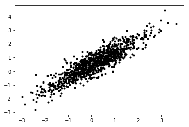
Let us consider again the multivariate normal objective. The functionality in this section is described in previous notebooks.

First, define some parameters and draw data.

dim = 2
num_obs = 1000

mean_true = np.random.random(dim)
cov_true = np.random.random((dim, dim))
cov_true = 0.1 * np.eye(dim) + np.full((dim, dim), 1.0)

x = np.random.multivariate_normal(mean=mean_true, cov=cov_true, size=(num_obs, ))
plt.plot(x[:, 0], x[:, 1], 'k.')

[<matplotlib.lines.Line2D at 0x7f030ffdeda0>]

Define paragami patterns and a loss function.

mvn_pattern = paragami.PatternDict(free_default=True)
mvn_pattern['mean'] = paragami.NumericVectorPattern(length=dim)
mvn_pattern['cov'] = paragami.PSDSymmetricMatrixPattern(size=dim)

# ``example_utils.get_normal_log_prob`` returns the log probability of
# each datapoint x up to a constant.
def get_loss(x, sigma, mu):
    return -1 * np.sum(
        example_utils.get_normal_log_prob(x, sigma, mu))

get_free_loss = paragami.FlattenFunctionInput(
    lambda mvn_par: get_loss(x=x, sigma=mvn_par['cov'], mu=mvn_par['mean']),
    patterns=mvn_pattern,
    free=True)

mvn_par = mvn_pattern.random()
mvn_free = mvn_pattern.flatten(mvn_par)

Optimization objectives.

We can use get_free_loss to define an optimization objective and pass it to scipy.optimize.minimize.

objective = paragami.OptimizationObjective(get_free_loss)

def Optimize(objective, x0=np.zeros(mvn_pattern.flat_length())):
    opt_result = sp.optimize.minimize(
        x0=x0,
        fun=objective.f,
        jac=objective.grad,
        hessp=objective.hessian_vector_product,
        method='trust-ncg')
    return opt_result

Controlling printing.

The frequency of printing can be controlled with set_print_every(), and the count can be reset with reset().

print('\nOptimizing:')
opt_result = Optimize(objective)
print(opt_result.message)

print('\nOptimizing printing less:')
objective.reset()
objective.set_print_every(5)
opt_result = Optimize(objective)
print(opt_result.message)

print('\nOptimizing without reset:')
opt_result = Optimize(objective)
print(opt_result.message)

print('\nOptimizing without printing:')
objective.set_print_every(0)
opt_result = Optimize(objective)
print(opt_result.message)

Optimizing:
Iter 0: f = 1290.22412134
Iter 1: f = 539.49481319
Iter 2: f = 449.15367362
Iter 3: f = 272.45823141
Iter 4: f = 255.05895262
Iter 5: f = 254.63015576
Iter 6: f = 254.47898697
Iter 7: f = 254.47819241
Iter 8: f = 254.47818845
Iter 9: f = 254.47818845
Optimization terminated successfully.

Optimizing printing less:
Iter 0: f = 1290.22412134
Iter 5: f = 254.63015576
Optimization terminated successfully.

Optimizing without reset:
Iter 10: f = 1290.22412134
Iter 15: f = 254.63015576
Optimization terminated successfully.

Optimizing without printing:
Optimization terminated successfully.

Accessing derivatives.

The function value and derivatives are methods of the optimization objective. Under the hood, all the derivatives are calcualted with autograd.

opt_x = opt_result.x

print('f() evaluates the objective:\n{} = {}'.format(
    objective.f(opt_x), get_free_loss(opt_x)))

grad = objective.grad(opt_x)
print('\ngrad() evaluates the gradient:\n{}'.format(grad))

print('\nhessian() evaluates the Hessian matrix:\n{}'.format(objective.hessian(opt_x)))

print('\nhessian_vector_product() evaluates the Hessian-vector product:\n{}'.format(
    objective.hessian_vector_product(opt_x, grad)))

f() evaluates the objective:
254.47818844774238 = 254.47818844774238

grad() evaluates the gradient:
[-9.38462682e-07 -8.28401150e-07  1.12731491e-06 -9.35645267e-07
  3.23708426e-06]

hessian() evaluates the Hessian matrix:
[[ 4.80152064e+03 -4.37310150e+03  9.83363903e-06 -6.91901344e-06
  -1.47624300e-06]
 [-4.37310150e+03  4.90797543e+03 -8.10149773e-06  8.64973804e-06
   1.65680224e-06]
 [ 9.83363896e-06 -8.10149785e-06  6.30553475e+03 -4.59689665e+03
  -1.75268882e-06]
 [-6.91901349e-06  8.64973810e-06 -4.59689665e+03  4.90797543e+03
   1.87129286e-06]
 [-1.47624310e-06  1.65680237e-06 -1.75268281e-06  1.87129159e-06
   1.99999999e+03]]

hessian_vector_product() evaluates the Hessian-vector product:
[-8.83365609e-04  3.82200615e-05  1.14093879e-02 -9.77427408e-03
  6.47416850e-03]

Logging.

By default, an optimization objective does no logging. But by using set_log_every with a number larger than 0, a log of the values is kept.

print('\nOptimizing with logging:')
objective.reset()
objective.set_print_every(0)
objective.set_log_every(2)
opt_result = Optimize(objective)
print(opt_result.message)

Optimizing with logging:
Optimization terminated successfully.

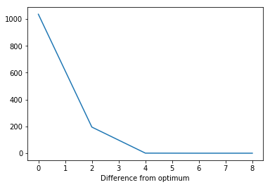
The log is contained in the attribute optimization_log. By default, each entry in the log is a tuple containing the iteration number, argument, and function value.

for log_entry in objective.optimization_log:
    print(log_entry)

plt.plot(
    [ entry[0] for entry in objective.optimization_log],
    [ entry[2] - opt_result.fun for entry in objective.optimization_log])
plt.xlabel('Iteration')
plt.xlabel('Difference from optimum')

(0, array([0., 0., 0., 0., 0.]), 1290.2241213426291)
(2, array([ 0.09798938,  0.57638205,  0.10194361,  0.92848007, -1.16334881]), 449.1536736241908)
(4, array([ 0.10983197,  0.58725075,  0.05844622,  0.94244548, -0.80874364]), 255.05895261654913)
(6, array([ 0.13464741,  0.61326864,  0.04907768,  0.9356453 , -0.7953923 ]), 254.47898697444145)
(8, array([ 0.13480492,  0.61343579,  0.04990915,  0.93661793, -0.79543076]), 254.4781884477883)

Text(0.5, 0, 'Difference from optimum')

The method reset() clears the log as well as the iteration count. Note that you can clear the log only using reset_log() and clear the iteration count only using reset_iteration_count().

objective.reset()
print(objective.optimization_log)

[]

Overloading.

Both the logging and progress methods can be overloaded to provide custom behavior.

class CustomObjective(paragami.OptimizationObjective):
    def print_value(self, num_f_evals, x, f_val):
        grad = objective.grad(x)
        print('Iteration {}: gradient norm = {:0.8f}'.format(
            num_f_evals, np.linalg.norm(grad)))

    def log_value(self, num_f_evals, x, f_val):
        grad = self.grad(x)
        self.optimization_log.append((num_f_evals, np.linalg.norm(grad)))

custom_objective = CustomObjective(get_free_loss)

print('\nOptimizing with custom printing and logging:')
custom_objective.reset()
custom_objective.set_print_every(1)
custom_objective.set_log_every(1)
opt_result = Optimize(custom_objective)
print(opt_result.message)

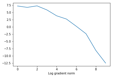
plt.plot(
    [ entry[0] for entry in custom_objective.optimization_log],
    np.log([ entry[1] for entry in custom_objective.optimization_log]))
plt.xlabel('Iteration')
plt.xlabel('Log gradient norm')

Optimizing with custom printing and logging:
Iteration 0: gradient norm = 1325.81210303
Iteration 1: gradient norm = 822.69307418
Iteration 2: gradient norm = 1380.15778047
Iteration 3: gradient norm = 343.45510333
Iteration 4: gradient norm = 44.95265409
Iteration 5: gradient norm = 14.74702496
Iteration 6: gradient norm = 1.23658409
Iteration 7: gradient norm = 0.09246396
Iteration 8: gradient norm = 0.00029502
Iteration 9: gradient norm = 0.00000377
Optimization terminated successfully.

Text(0.5, 0, 'Log gradient norm')